Text classification from BOW to Transformers (1)

#machine-learning #text-classification #natural-language-processing

Text Classification: From Bag of Words (BOW) to Transformers

Text classification is a core task in natural language processing (NLP) that involves categorizing text into predefined labels or categories. This process is used across many applications, such as sentiment analysis, spam detection, language identification, and topic categorization.

In this blog post, we’ll walk through the progression of text classification methods, starting from the basic Bag of Words (BOW) model, moving through TF-IDF, XGBoost, and concluding with deep learning models such as CNNs, RNNs, and Transformers. By examining each of these techniques, you will understand the pros and cons of each and gain a solid foundation for choosing the right model for your task.

For this post, we’ll use the IMDB movie reviews dataset from Hugging Face’s dataset repository to showcase the implementation and evaluation of each method. You can find the dataset here.

Introduction to Text Classification

At its core, text classification assigns a label to a piece of text. For example, given a movie review, a text classification model can predict whether the review is positive or negative.

A typical pipeline for text classification includes the following steps:

Preprocessing: Clean and tokenize the text.
Feature Extraction: Convert the text into a numerical representation that machine learning models can interpret.
Model Training: Train the model on labeled text data to learn the mapping between text and labels.
Evaluation: Measure the model’s performance on test data.
Prediction: Use the trained model to predict labels for new data.

There are different approaches to each of these steps, and over the years, various techniques have been introduced to improve the classification performance. Let’s start with the Bag of Words (BOW) model.

Bag of Words (BOW) Model

What is BOW?

Bag of Words (BOW) is one of the simplest techniques for text classification. It represents text as an unordered collection of words, completely ignoring word order and treating each word as an independent feature. Each word in the text is represented by its frequency in the document.

For example, given two sentences:

"The dog chased the cat."
"The cat chased the dog."

The BOW representation will treat both sentences the same, because it ignores word order. This leads to some key limitations, which we’ll discuss shortly.

Limitations of BOW

No Context or Word Order: The BOW model loses important information by ignoring word order. For instance, "The dog chased the cat" is different from "The cat chased the dog," but BOW would treat them identically.
High Dimensionality: Each unique word is treated as a feature, leading to high-dimensional feature spaces, which can be computationally expensive.
Sparse Representation: Since most documents only contain a small fraction of the entire vocabulary, the resulting feature matrix is sparse (containing many zeros).

Implementing BOW

Let’s now see how to implement the Bag of Words model using the IMDB movie reviews dataset. First, we load the dataset and inspect it.

import pandas as pd

# Load the dataset
splits = {'train': 'IMDB_train.csv', 'validation': 'IMDB_validation.csv', 'test': 'IMDB_test.csv'}
train_df = pd.read_csv("hf://datasets/jahjinx/IMDb_movie_reviews/" + splits["train"])
test_df = pd.read_csv("hf://datasets/jahjinx/IMDb_movie_reviews/" + splits["test"])
valid_df = pd.read_csv("hf://datasets/jahjinx/IMDb_movie_reviews/" + splits["validation"])

# Example review and label
print(f"text :{train_df.iloc[0,0]}")
print(f"label :{train_df.iloc[0,1]}")

text :Beautifully photographed and ably acted, generally, but the writing is very slipshod. There are scenes of such unbelievability that there is no joy in the watching. The fact that the young lover has a twin brother, for instance, is so contrived that I groaned out loud. And the "emotion-light bulb connection" seems gimmicky, too.

I don't know, though. If you have a few glasses of wine and feel like relaxing with something pretty to look at with a few flaccid comedic scenes, this is a pretty good movie. No major effort on the part of the viewer required. But Italian film, especially Italian comedy, is usually much, much better than this.
label :0

Each review in the dataset has a corresponding label (0 for negative, 1 for positive). Next, we’ll preprocess the data.

Preprocessing and Vectorization

We will clean the text by removing punctuation, converting the text to lowercase, and tokenizing it into words. Afterward, we will use CountVectorizer from the scikit-learn library to create a Bag of Words representation of the text.

import re
from sklearn.feature_extraction.text import CountVectorizer
from nltk.tokenize import word_tokenize

# Preprocess function to clean text
def clean_text(text):
    return re.sub(r"[^\w\s+]", '', text)

# Initialize CountVectorizer for BOW representation
vectorizer = CountVectorizer(lowercase=True, preprocessor=clean_text,
                             tokenizer=word_tokenize, stop_words='english', max_features=300)

# Fit and transform the training data
train_text_array = vectorizer.fit_transform(train_df['text'])
test_text_array = vectorizer.transform(test_df['text'])

The output of the above code gives a sparse matrix where each row represents a document (movie review), and each column represents a word from the vocabulary (with a maximum of 300 words). The matrix stores the frequency of words in each document.

Classification with Logistic Regression

Now, we will use Logistic Regression to classify the reviews as positive or negative based on the Bag of Words representation.

from sklearn.linear_model import LogisticRegression
from sklearn.metrics import classification_report

# Train logistic regression model
model = LogisticRegression()
model.fit(train_text_array, train_df['label'].values)

# Predict and evaluate on the test set
preds = model.predict(test_text_array)
print("Accuracy: ", model.score(test_text_array, test_df['label'].values))
print(classification_report(test_df['label'].values, preds))

Results

Metric	Precision	Recall	F1-Score	Support
Negative (0)	0.81	0.77	0.79	5044
Positive (1)	0.78	0.81	0.80	4956
Accuracy			0.79	10000

As we can see, the Bag of Words model performs reasonably well, achieving an accuracy of around 79%. However, there is room for improvement, especially in capturing the semantic meaning and context of the text. This is where TF-IDF comes into play.

TF-IDF with Logistic Regression

What is TF-IDF?

TF-IDF (Term Frequency-Inverse Document Frequency) is a more refined version of BOW. It calculates the importance of a word by considering how frequently it appears in a document (TF) and how unique it is across all documents in the corpus (IDF). Words that appear frequently but are not common across many documents receive higher weights, allowing TF-IDF to better capture the importance of specific words.

The formula for TF-IDF is:

TF-IDF (t, d) = TF (t, d) \times \log (\frac{N}{DF (t)})

Where:

TF(t, d): Term frequency, the number of times term t appears in document d.
DF(t): Document frequency, the number of documents that contain the term t.
N: Total number of documents.

Implementing TF-IDF

We will now apply TF-IDF to the movie review dataset using TfidfVectorizer from scikit-learn.

from sklearn.feature_extraction.text import TfidfVectorizer

# Apply TF-IDF transformation
tfidf_vectorizer = TfidfVectorizer(lowercase=True, preprocessor=clean_text,
                                   tokenizer=word_tokenize, stop_words='english', max_features=300)
train_text_tfidf = tfidf_vectorizer.fit_transform(train_df['text'])
test_text_tfidf = tfidf_vectorizer.transform(test_df['text'])

# Train and evaluate logistic regression
model.fit(train_text_tfidf, train_df['label'].values)
preds = model.predict(test_text_tfidf)
print("Accuracy: ", model.score(test_text_tfidf, test_df['label'].values))
print(classification_report(test_df['label'].values, preds))

Results

Metric	Precision	Recall	F1-Score	Support
Negative (0)	0.81	0.78	0.79	5044
Positive (1)	0.78	0.81	0.80	4956
Accuracy			0.79	10000

TF-IDF achieves nearly the same performance as Bag of Words. However, TF-IDF often performs better on larger and more complex datasets by giving more weight to important but rare words.

Gradient Boosting with XGBoost

XGBoost is a popular machine learning algorithm that uses gradient boosting. It is known for its high performance in many machine learning competitions and its ability to handle large datasets efficiently. By iteratively improving weak learners (usually decision trees), XGBoost creates a strong model.

XGBoost can handle sparse input data, making it a good fit for text classification using BOW or TF-IDF features.

Implementing XGBoost

We will train an XGBoost model on the TF-IDF features of the movie reviews.

import xgboost as xgb

# Prepare data in DMatrix format
dtrain = xgb.DMatrix(train_text_tfidf, label=train_df['label'].values)
dtest = xgb.DMatrix(test_text_tfidf, label=test_df['label'].values)

# Define model parameters
param = {'max_depth': 6, 'eta': 0.3, 'objective': 'binary:logistic'}
num_round = 10

# Train XGBoost model
import xgboost as xgb
from ray import train, tune
from ray.tune.schedulers import ASHAScheduler
from ray.tune.integration.xgboost import TuneReportCheckpointCallback

def train_model(config,train_x,train_y,test_x,test_y):
    dtrain = xgb.DMatrix(train_x,label=train_y)
    dtest = xgb.DMatrix(test_x,label=test_y)
    results = {}
    bst = xgb.train(config,
                    dtrain,
                    num_boost_round=10,
                    evals=[(dtest,'test')],
                    evals_result=results,
                    callbacks=[TuneReportCheckpointCallback(frequency=1)]
                    )
    accuracy = 1-results['test']['error'][-1]
    train.report({"Mean Accuracy": accuracy, "done": True})

def get_best_model_checkpoint(results):
    best_result = results.get_best_result()
    best_bst = TuneReportCheckpointCallback.get_model(best_result.checkpoint)
    accuracy = 1-best_result.metrics['test-error']
    print(f"Best model parameters: {best_result.config}")
    print(f"Best model found has an accuracy of {accuracy:4f}")
    return best_bst


def tune_model(train_x,train_y,test_x,test_y,smoke_test=False):
    search_space = {
        'objective':'binary:logistic',
        'eval_metric': ['error','logloss'],
        'max_depth': tune.randint(1,9),
        'max_child_weight': tune.choice([1,2,3]),
        'subsample': tune.uniform(0.5,1),
        'eta': tune.loguniform(1e-4,1e-1),
    }

    scheduler = ASHAScheduler(
        max_t=10,
        grace_period=1,
        reduction_factor=2
    )

    tuner = tune.Tuner(
        tune.with_parameters(train_model,
                            train_x=train_x,
                            train_y=train_y,
                            test_x=test_x,
                            test_y=test_y),
        tune_config=tune.TuneConfig(metric="test-logloss",
                                    mode="min",
                                    scheduler=scheduler,
                                    num_samples= 1 if smoke_test else 100,
                                    ),
        param_space=search_space

    )

    results = tuner.fit()
    return results

results = tune_model(
    train_text_array,
    train_df['label'].values,
    test_text_array,
    test_df['label'].values,
    smoke_test=False
)

Results

Accuracy: 71.7%

XGBoost performs worse than logistic regression in this case, but it may excel on other datasets or with more in depth hyperparameter tuning.

Deep Learning Models: CNNs and RNNs

Traditional models like Logistic Regression and XGBoost are limited in their ability to capture the sequential nature of text. Deep learning models, particularly Convolutional Neural Networks (CNNs) and Recurrent Neural Networks (RNNs), can automatically learn patterns in text and account for both local and global dependencies.

CNNs are good at detecting local patterns, such as word n-grams.
RNNs can capture long-range dependencies and are excellent for modeling sequences.

Convolutional Neural Networks (CNNs)

A CNN applies filters across the text to detect patterns such as combinations of words. These patterns are then used for classification.

import torch
import torch.nn as nn
import torch.optim as optim
from torch.utils.data import DataLoader, TensorDataset

# Define CNN model
class CNNClassifier(nn.Module):
    def __init__(self, input_dim):
        super(CNNClassifier, self).__init__()
        self.conv1 = nn.Conv1d(in_channels=1, out_channels=128, kernel_size=3)
        self.fc1 = nn.Linear(128, 1)

    def forward(self, x):
        x = self.conv1(x.unsqueeze(1))
        x = torch.relu(x)
        x = torch.max(x, 2)[0]
        x = self.fc1(x)
        return x

Recurrent Neural Networks (RNNs)

RNNs are designed to handle sequential data. They can maintain information about previous words in the sequence, which helps them capture dependencies in text.

class RNNClassifier(nn.Module):
    def __init__(self, input_dim):
        super(RNNClassifier, self).__init__()
        self.rnn = nn.RNN(input_dim, 128, 2, batch_first=True)
        self.fc1 = nn.Linear(128, 1)

    def forward(self, x):
        _, hn = self.rnn(x.unsqueeze(1))
        x = self.fc1(hn[-1])
        return x

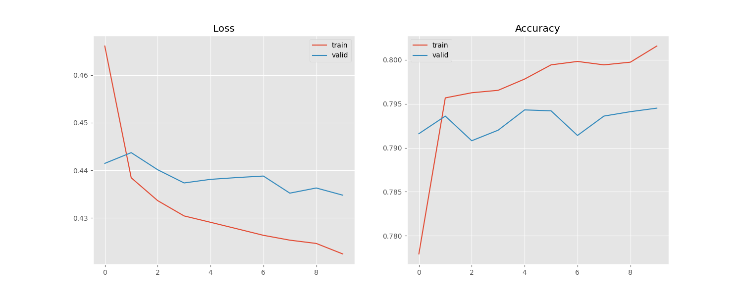
Results of CNN and RNN

Model	Accuracy
CNN	53.9%
RNN	79.4%

RNNs perform significantly better than CNNs in this case, likely due to their ability to model the sequential nature of text more effectively and the performance of RNN is along the lines of the logistic regression model.

The poor performance of the CNN model is expected, we may see improvement by using n-grams instead of single words

rnn

The Transformer Era

Transformers revolutionized NLP by introducing the self-attention mechanism, which allows models to capture long-range dependencies in text more efficiently than RNNs. Models like BERT and GPT are built on the transformer architecture and have set new benchmarks in NLP tasks.

Transformers are capable of:

Understanding context better: They capture both local and global relationships in the text.
Scaling better: Transformers can be trained in parallel, unlike RNNs which process sequences one step at a time.

We will explore transformers like BERT and GPT in the next blog post and learn how to implement them for text classification.

Conclusion and Next Steps

In this blog post, we walked through the progression of text classification techniques:

Bag of Words (BOW): Simple but loses word order and context.
TF-IDF: Adds importance to rare but significant words.
XGBoost: A strong boosting algorithm that handles sparse data.
Deep Learning (CNNs and RNNs): Models that capture local and sequential patterns.
Transformers: The state-of-the-art models for NLP.

Each technique offers different advantages, but the choice of model depends on the task at hand. Transformers represent the cutting edge of NLP and are typically the best choice for complex text classification tasks.

In the next post, we will explore transformers like BERT and GPT in detail and learn how to implement them for text classification. We’ll also dive into the concept of word embeddings and how they enhance deep learning models in NLP.

Stay tuned!