Understanding Overfitting in Machine Learning

#machine-learning #overfitting #regularization

One of the key objectives in machine learning is to develop models that generalize well to new, unseen data. However, a frequent challenge is overfitting, where a model becomes excessively tailored to the training data, capturing noise instead of the underlying pattern. This blog explores the concept of overfitting, the impact of data size on overfitting, and how regularization techniques can mitigate overfitting to create more robust models.

Building a Simple Regression Model

To illustrate overfitting, let's start with a simple regression problem. Suppose we observe a real-valued input variable $x$ and wish to predict the value of a real-valued target variable $t$ . For clarity, we'll use synthetically generated data because the exact process that generated the data is known, making it easier to compare against any learned model.

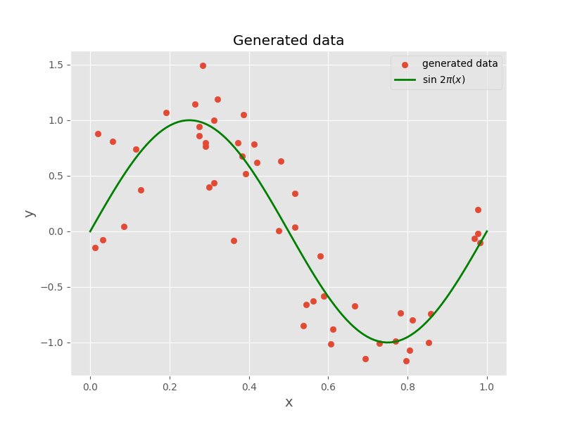
We generate synthetic data using the function $\sin (2 π x)$ with some added Gaussian noise. Below is a plot of 50 data points generated using this process:

initial generated data

Our goal is to use this training set to predict the value $\hat{t}$ of the target variable for some new value $\hat{x}$ of the input variable. This involves implicitly trying to discover the underlying function $\sin (2 π x)$ .

Curve Fitting with Polynomial Functions

We will approach this problem by fitting the data using a polynomial function of the form:

y (x, w) = w_{0} + w_{1} x + w_{2} x^{2} + \dots + w_{M} x^{M} = \sum_{j = 0}^{M} w_{j} x^{j}

where $w = (w_{0}, w_{1}, \dots, w_{M})^{T}$ are the model parameters. The polynomial is of order $M$ , and we refine the fit by adjusting the parameters $w$ to minimize an error function, specifically the sum of squares of the errors between the predictions $y (x, w)$ and the corresponding target values $t$ :

E (w) = \frac{1}{2} \sum_{n = 1}^{N} {y (x_{n}, w) - t_{n}}^{2}

Here, $N$ is the number of data points. The factor $\frac{1}{2}$ is included for convenience. Although the sum-of-squares error function is commonly used, other error functions may be more appropriate depending on the context.

The solution to this curve fitting problem involves finding the value of $w$ that minimizes the error function $E (w)$ . Since the error function is quadratic in $w$ , it is convex and has a unique minimum, which can be found by setting the derivatives of $E (w)$ with respect to $w$ to zero. The resulting polynomial is denoted by $y (x, w^{*})$ .

Exploring the Effect of Polynomial Order on Model Fit

To understand overfitting, we examine how the order of the polynomial affects model fit. We fit polynomials of different orders to the training data and observe the results. Additionally, we evaluate the models on new, unseen data to assess their generalization ability.

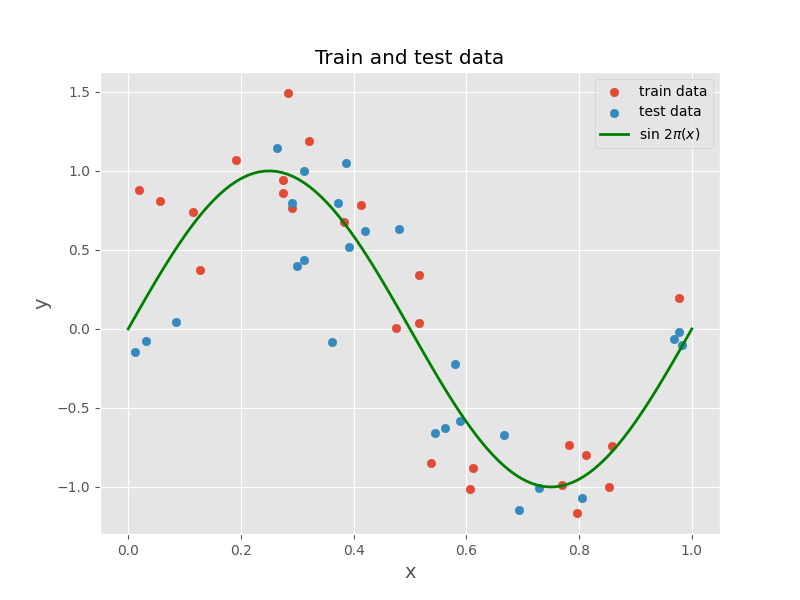
We start by dividing our data into training and test sets. The training set is used to fit the model, while the test set is used to evaluate the model's performance.

training and test data

By fitting polynomials of varying orders to the training data and using the mean squared error (MSE) as our evaluation metric, we can observe how the model's complexity impacts its performance.

polynomial fits

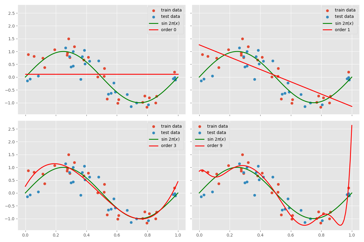
As the order of the polynomial increases, the model becomes more complex and fits the training data more closely. However, this increased complexity may lead to overfitting, where the model captures noise in the training data instead of the underlying pattern. In the plot above, the polynomial of order 9 oscillates excessively to capture the noise, whereas the polynomial of order 1 is too simple to capture the underlying pattern. The polynomial of order 3, on the other hand, seems to strike a balance by capturing the underlying pattern effectively.

Evaluating Model Performance

To further analyze the impact of polynomial order on model performance, we plot the training and test errors as a function of polynomial order. The training error decreases as the polynomial order increases because the model becomes more complex and fits the training data more closely. However, the test error initially decreases and then increases as the model becomes too complex and begins to overfit the training data. The optimal model complexity is the one that minimizes the test error, as it generalizes well to new data.

We use the root mean squared error (RMSE) as a metric for evaluating model performance, defined as the square root of the average of the squared differences (MSE) between the predicted values and the true values.

rmse vs polynomial order

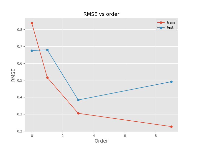
The plot above shows that the test error is minimized for a polynomial of order 3, which captures the underlying pattern without overfitting the training data. This demonstrates the trade-off between model complexity and generalization performance and highlights the importance of choosing the appropriate model complexity to avoid overfitting.

The output below summarizes the RMSE for different polynomial orders on both the training and test data:

Order: 0, RMSE (train): 0.8381, RMSE (test): 0.6753
Order: 1, RMSE (train): 0.5162, RMSE (test): 0.6796
Order: 3, RMSE (train): 0.3547, RMSE (test): 0.3835
Order: 9, RMSE (train): 0.2265, RMSE (test): 0.4911

As shown, the RMSE for the test data is minimized for a polynomial of order 3.

Analyzing Polynomial Coefficients

We can gain further insights by examining the coefficients of the polynomial for different orders:

Order: 0, Coefficients: [0.11941504]
Order: 1, Coefficients: [ 0.06102459 -1.15146493]
Order: 3, Coefficients: [-0.06511999 -2.69902699  0.36666158  2.55591654]
Order: 9, Coefficients: 
[ 1.08414773e-02 -4.17947771e+00 -2.45869645e+00  7.26680257e+00
  1.52424608e+01  9.83486762e+00 -2.99539542e+01 -3.50059274e+01
  1.77062867e+01  2.17339983e+01]

As the polynomial order increases, the magnitude of the coefficients generally becomes larger. For the polynomial of order 9, the coefficients are finely tuned to the data, developing large positive and negative values to match each data point exactly.

Techniques to Reduce Overfitting

Increasing Data Size

One way to reduce overfitting is to use more data. As the number of data points increases, the model has more information to learn the underlying pattern, reducing the likelihood of overfitting. We can observe this by generating more data points and fitting polynomials of different orders to the new data.

more data

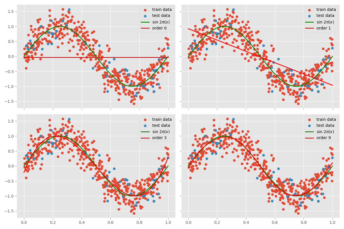
With more data points, the polynomial of order 9 fits the data more closely without overfitting, as it has more information to learn the underlying pattern. This highlights the importance of having sufficient data to train complex models.

Applying Regularization

Another effective technique to reduce overfitting is regularization, which adds a penalty term to the error function to discourage overly complex models. Regularization techniques, such as L1 and L2 regularization, penalize large coefficients and promote simpler models.

For example, L2 regularization modifies the error function as follows:

E (w) = \frac{1}{2} \sum_{n = 1}^{N} {y (x_{n}, w) - t_{n}}^{2} + \frac{λ}{2} | | w | |^{2}

Here, $λ$ is the regularization parameter that controls the strength of the penalty term. By adjusting $λ$ , we can balance the trade-off between fitting the data and maintaining model simplicity.

The Impact of Regularization

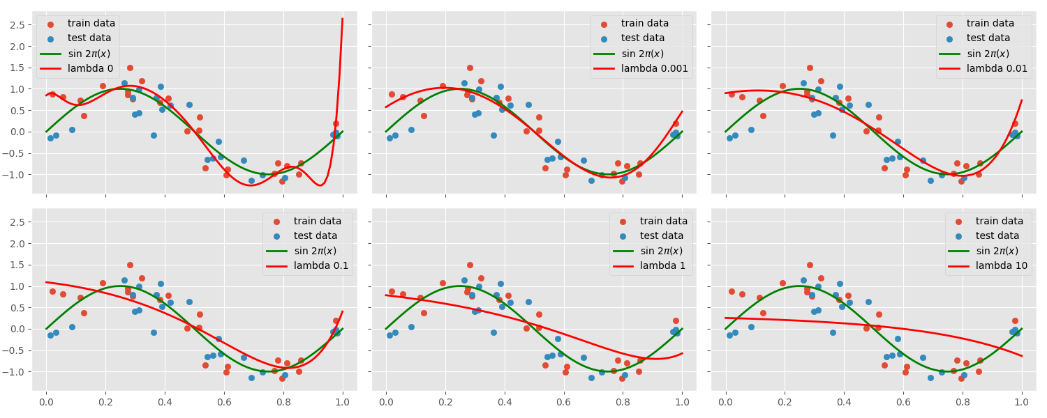
To see how regularization affects model complexity, we apply L2 regularization with different values of $λ$ to the polynomial of order 9 from the initial data:

regularization

As $λ$ increases, the model becomes simpler and less prone to overfitting, as the penalty term discourages large coefficients. This demonstrates how regularization can help reduce overfitting and promote simpler models that generalize well.

While regularization can help prevent overfitting, it is crucial to choose an appropriate value for $λ$ . Cross-validation is a common technique used to select the optimal $λ$ by evaluating the model's performance on validation data. By tuning the regularization parameter using cross-validation, we can select a model that generalizes well to new, unseen data.

Conclusion

Overfitting is a common challenge in machine learning, where a model becomes too tailored to the training data, capturing noise instead of the underlying pattern. This can be mitigated by increasing the amount of training data and applying regularization techniques, such as L1 and L2 regularization, which penalize overly complex models. By selecting the appropriate model complexity and regularization parameters, we can create models that generalize well and are robust to noise in the training data.

Resources :

[Pattern Recognition and Machine Learning-Bishop](Pattern Recognition and Machine Learning)
code for generating the data and fitting the models can be found here